
Page 15 - Code Craft Computer-7
P. 15
CELL RANGE
A cell range in Excel can be defined as a group of selected cells. A cell range can be used to
perform calculation on multiple cells. You can create a range either by selecting the continuous
cells in a worksheet or using the colon (:) symbol. Let us learn how to select a range of cells.
• Consider the worksheet given here.
• Click inside cell A1 and drag the mouse pointer till cell D6.
• You can observe that all the cells are selected.
• This range that is selected here can be denoted as 'A1:D6'.
Using a Range
You can use a range in a function. For example, if you want to calculate the sum of multiple
columns or rows, it is always better to define a range. Follow the given steps to use a range in a
formula:
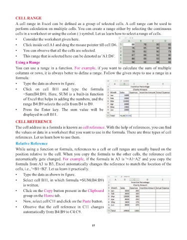
• Type the data as shown in figure.
• Click on cell B11 and type the formula
=Sum(B4:B9). Here, SUM is a built-in function
of Excel that helps in adding the numbers, and the
range B4:B9 selects the cells from B4 to B9.
• Press the Enter key. The sum value will be
displayed in cell B11.
CELL REFERENCE
The cell address in a formula is known as cell reference . With the help of references, you can find
the values or data in a worksheet that you want to use in the formula. There are three types of cell
references. Let us learn how to use them.
Relative Reference
While using a function or formula, references to a cell or cell ranges are usually based on the
position relative to the cell. When you copy the formula to the other cells, the reference cell
automatically gets changed. For example, if the formula in A3 is '=Al+A2' and you copy the
formula from A3 to B3, Excel automatically changes the reference to match the location of the
cells, i.e., '=B1+B2'. Let us learn it practically.
• Type the data as shown in figure.
• Select cell B11, in which formula =SUM(B4:B9)
is written.
• Click on the Copy button present in the Clipboard
group on the Home tab.
• Now, select cell C11 and click on the Paste button.
• Observe that the cell reference in C11 changes
automatically from B4:B9 to C4:C9.
15