
Page 52 - Code Craft Computer-7
P. 52
PIVOTTABLE
PivotTable is a powerful tool for consolidating, summarising and presenting data. To create
PivotTables, follow these steps:
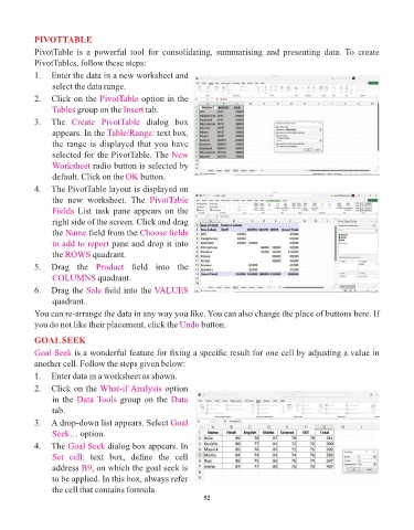
1. Enter the data in a new worksheet and
select the data range.
2. Click on the PivotTable option in the
Tables group on the Insert tab.
3. The Create PivotTable dialog box
appears. In the Table/Range: text box,
the range is displayed that you have
selected for the PivotTable. The New
Worksheet radio button is selected by
default. Click on the OK button.
4. The PivotTable layout is displayed on
the new worksheet. The PivotTable
Fields List task pane appears on the
right side of the screen. Click and drag
the Name field from the Choose fields
to add to report pane and drop it into
the ROWS quadrant.
5. Drag the Product field into the
COLUMNS quadrant.
6. Drag the Sale field into the VALUES
quadrant.
You can re-arrange the data in any way you like. You can also change the place of buttons here. If
you do not like their placement, click the Undo button.
GOAL SEEK
Goal Seek is a wonderful feature for fixing a specific result for one cell by adjusting a value in
another cell. Follow the steps given below:
1. Enter data in a worksheet as shown.
2. Click on the What-if Analysis option
in the Data Tools group on the Data
tab.
3. A drop-down list appears. Select Goal
Seek… option.
4. The Goal Seek dialog box appears. In
Set cell: text box, define the cell
address B9 , on which the goal seek is
to be applied. In this box, always refer
the cell that contains formula.
52