Page 53 - Code Craft Computer-7

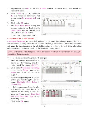
5. Type the new value 405 as a result in To value : text box. In this box, always refer the cell that
contains formula.

6. Press the Tab key and click on the cell
E3 in a worksheet. The address will
appear in the By changing cell: text
box.
7. Click on the OK button.

8. The Goal Seek Status dialog box
appears on the screen displaying the
Target value 405 and Current value
392. Click on the OK button.

Observe the change in the cell E5.

CONDITIONAL FORMATTING
Conditional formatting is a feature in Excel that lets you apply formatting such as cell shading or
font colour to a cell only when the cell contents satisfy a given condition. When the value of the

cell meets the format condition, the selected formatting is applied to the cell. If the value of the
cell does not meet the format condition, the default formatting is used.

Note : Conditional formatting is a feature that allows you to set a cell’s format according to
conditions that you specify.

To apply conditional formatting, follow these steps:

1. Enter the data in a new worksheet as
shown and select the range of cells to
be formatted (for example , B2: F7 ).
2. Click on the Conditional Formatting

option in the Styles group on the
Home tab. A list of options is
displayed.
3. Select the required option as per the
criteria you want to apply. Here we
select Highlight Cells Rules >

Greater Than.
4. A dialog box appears. Enter the value
and specify the formatting to be
applied. In this example, enter the

value as 85 and choose Light Red
Fill with Dark Red Text as the
formatting option.
5. Click on the OK button.

53